We can parameterize the constraint, i.e
Now stick it into to get To find max (or min):
Which makes (see quotient identities), the critical points are at . Critical points: , so the critical points are:
We can look at the derivative. Observe:
**The extrema occur at the points** where the constraint curve and level curves **touch tangentially**. Using the chain rule for paths:
$$
\begin{align}
\frac{dg}{dt} & = \frac{d}{dt}f\big(x(t), y(t)\big) \\
& = \frac{ \partial f }{ \partial x } \frac{dx}{dt} + \frac{ \partial f }{ \partial y } \frac{dy}{dt} \\
& = \vec{\nabla}f \cdot \frac{d\vec{r}}{dt} \\
& = 0
\end{align}
$$
Recall that the Gradient Vector is orthogonal to the level curves, and the dot product of two orthogonal vectors is 0.
We know at the max, level curve is parallel to the constraint
Flip this idea around: a vector perpendicular to the level curve is perpendicular to constraint
Method of Lagrange
Definition
To find critical points of subject to the constraint , find so that
for some constant (Lagrange multiplier).
Example
Same example, find the max of subject to the constraint .
solution
We have , and . However, , so we have to go with the first case.
Next, , so and .
which means
and with , we have 3 equations with 3 unknowns.
Generally, we should just eliminate (since we don't need it again), and solve for and
sub this into our bounds:
So our critical points are:
Example
Find maximum of subject to
solution
Eliminate ,
so Is a (the only) critical point with the constraint.
Example
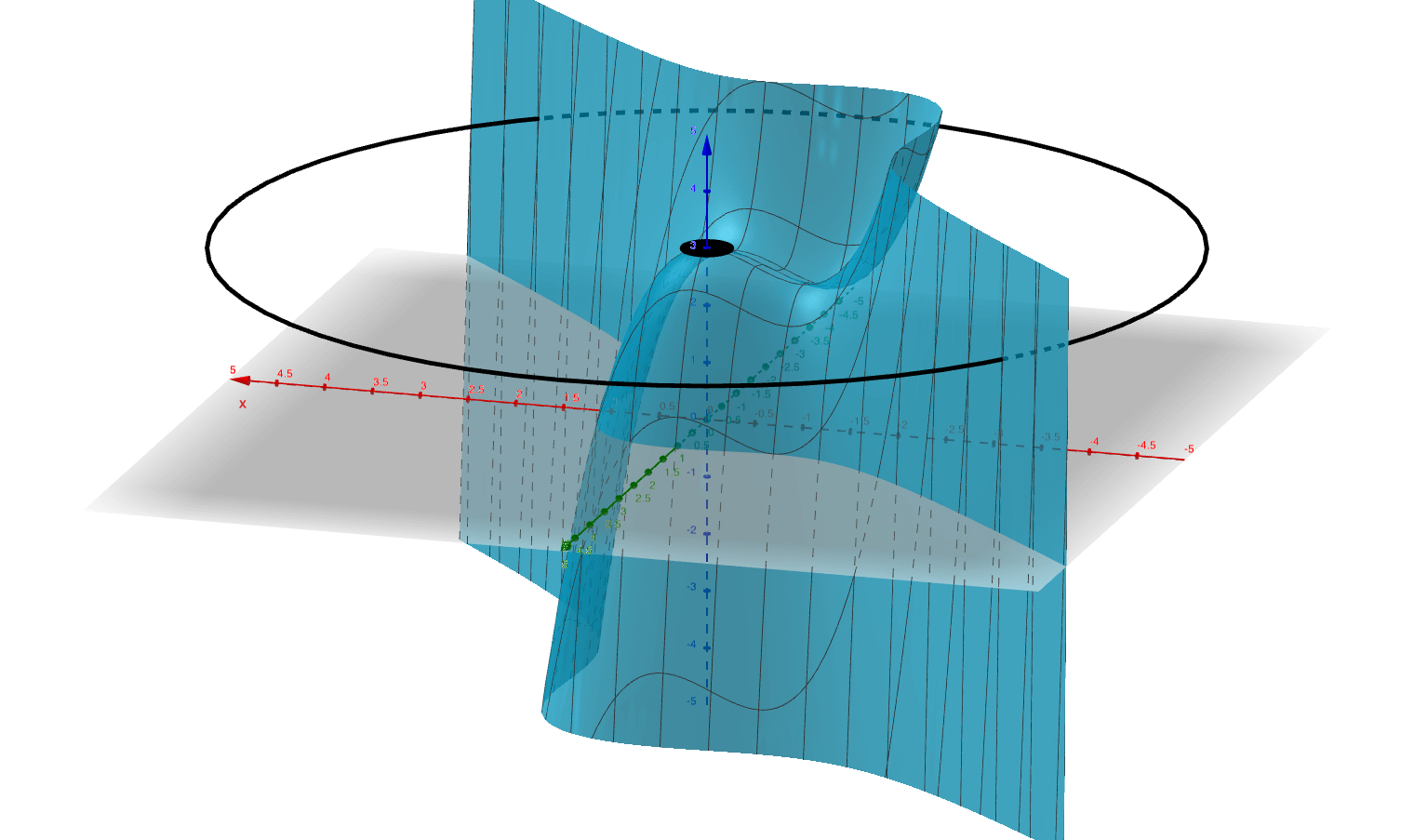
A circular hot plate given by the relationship is heated according to the spatial temperature function . Find the hottest and coldest temperatures on the plate and the points at which they occur.
solution
Let , .
We have:
First, to find the critical points on the boundary, we use the method of Lagrange:
We have , but , so we must use the Lagrange multiplier and solve the system.
We have , which gives the system:
Right away from , we can see is a possibility, which gives .
Then, solving by substitution, we find:
Plugging this in to , we find:
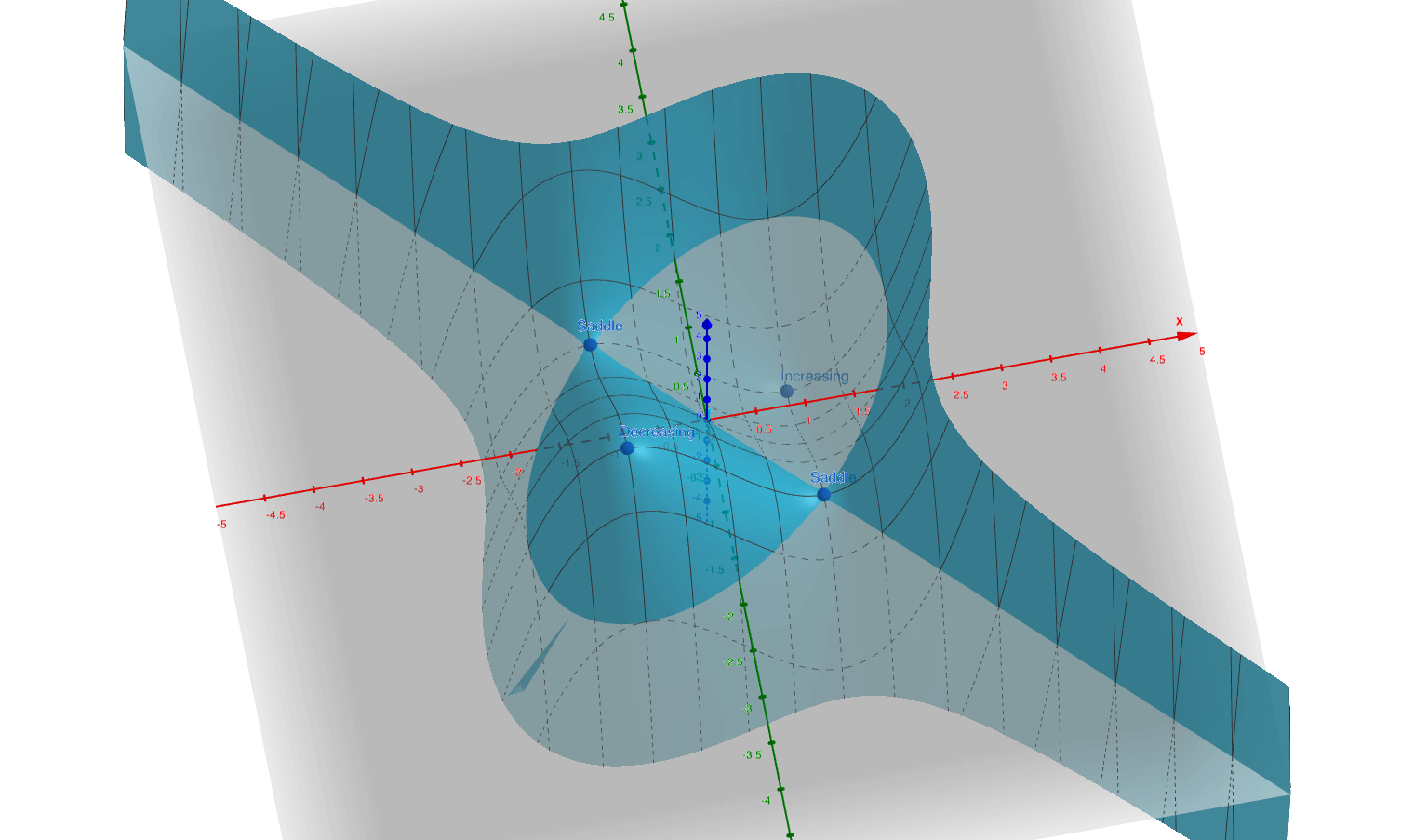
So our critical points on the boundary are , , , and .
Next, we have to check inside the boundary. For this, we perform unconstrained optimization and then check if the points we find are within the boundary.
We seek , which means:
This system is easy to solve; and .
In summary, our entire collection of critical points is , , , , and .
Now we plug in to to see which max/min:
Thus, the hot plate is hottest at with temperature , and is coldest at with temperature .